Model Order Reduction with External Solver

This example shows a harmonic analysis of a beam bending with both ends fixed using, using model order reduction to reduce the dimensions of the problem and save runtime. Since model order reduction is not yet implemented in openCFS, one has to use the external solver (Pyhton Script). In order to compare the solution of the reduced model, the computation is additionally done with the full model. Here you can download the files for this example:

• XML file for the eigenfrequency analysis (click here)
• XML file for the harmonic analysis with model order reduction (click here)
• XML file for the harmonic analysis with the full model (click here)
• Python script for the external solver (click here)
• Mesh input file for cubit (click here) and the mesh (click here)
• XML file for the material data (click here)
• Python script for the postprocessing (click here)

Setup

We conisder a beam of steel, which is fixed on both ends. On the blue region a pressure is applied.

After the discretisation with the Finite Element Method, the mechanical system leads to a second order linaear differential equation, with the system matrices $\mathbf{M}, \mathbf{D}, \mathbf{K} \in \mathbb{R}^{n\times n}$ (mass, damping and stiffness matrix) and the forcing vector $\mathbf{F}(t)\in \mathbb{R}^{n\times 1}$:

$$\begin{equation} \mathbf{M\ddot{u}}+\mathbf{D\dot{u}}+\mathbf{Ku}=\mathbf{F}(t) \label{eq:system_equation} \end{equation}$$

Model Order Reduction

The homogenous form of equation \eqref{eq:system_equation} with an harmonic approach $\mathbf{u}(t)=\mathbf{\psi} e^{j\omega t}$ leads to quadratic eigenvalue problem of the form

$$\begin{equation} (\mathbf{K}+j\omega \mathbf{D}-\omega^2 \mathbf{M})\mathbf{\psi}=\mathbf{0} \label{eq:quadratic_EVP} \end{equation}$$

with the eigenfrequencies $\omega_i$ and the corresponding eigenmodes $\mathbf{\psi}_i$. We now introduce the modal coordinates $q_i$ which represent the system with the linear transformation

$$\begin{equation} \mathbf{u} = \sum_{i=1}^{n} \mathbf{\psi}_i q_i = \mathbf{\Psi q} \label{eq:modal_coordinates} \end{equation}$$

in the form

\begin{equation} \mathbf{\bar{M}\ddot{q}}+\mathbf{\bar{C}\dot{q}}+\mathbf{\bar{K}q}=\mathbf{\bar{F}}(t) \label{eq:modal_system} \end{equation}

with the modal system matrics $\mathbf{\bar{M}}=\mathbf{\Psi^TM\Psi}$, $\mathbf{\bar{D}}=\mathbf{\Psi^TD\Psi}$, $\mathbf{\bar{K}}=\mathbf{\Psi^TK\Psi}$ and $\mathbf{\bar{F}}=\mathbf{\Psi^TF}$. Note, that the transformed system matrices are diagonal and if the eigenvectors are mass normalized, $\mathbf{\bar{M}}$ becomes the identity matrix.

If we only take sub-set $m$ of the $n$ modes, with $m<n$,

$$\begin{equation} \mathbf{u} = \sum_{i=1}^{m} \mathbf{\psi}_i q_i = \mathbf{\Psi_R q_R} \label{eq:reduced_modal_coordinates} \end{equation}$$

we can reduce the system order to $m$ and approximate the global system dynamics. The reduced model is given by equation \eqref{eq:modal_system} with $\mathbf{\bar{M}}=\mathbf{\Psi_R^TM\Psi_R}$, $\mathbf{\bar{D}}=\mathbf{\Psi_R^TD\Psi_R}$, $\mathbf{\bar{K}}=\mathbf{\Psi_R^TK\Psi_R}$, $\mathbf{\bar{F}}=\mathbf{\Psi_R^TF}$ and $\mathbf{q}=\mathbf{q_R}$. The choice of the sub-set of the modes depends on the frequency range of intereset and on the excitation, because not every exictation excites all modes.^{1 2 3}

Eigenfrequency Analysis

The eigenanalysis is done similiar as it is done in the tutorial of the Cantilever. For this example the first 10 eigenfrequencies and modes are calulated. Additionally the caclulated modes, mass, damping and stiffness matrices are exported in the Matrix Market format. In order to make sure that the order of the nodes is the same in the eigenfrequency and harmonic analysis, no reordering is allowed.

<solutionStrategy>
    <standard>
        <exportLinSys format="matrix-market" system="false" rhs="false" solution="true" mass="true" damping="true" stiffness="true" baseName="mode"/>
        <matrix reordering="noReordering"/>
    </standard>
</solutionStrategy> 

The results of the eigenfrequency analysis:

click to see the results of the eigenfrequency analysis

Mode 1 (52.4252 Hz)	Mode 2 (103.757 Hz)

Mode 3 (144.385 Hz)	Mode 4 (282.713 Hz)

Mode 5 (284.992 Hz)	Mode 6 (466.594 Hz)

Mode 7 (555.952 Hz)	Mode 8 (695.586 Hz)

Mode 9 (913.063 Hz)	Mode 10 (969.026 Hz)

Harmonic Analysis with Reduced Model

The harmonic analysis is done at 10 frequencies, equally sampled between 1 Hz and 1000 Hz. The Model Order Reduction will be done with the modes: 1, 3, 4, 6, 8, 10. Since we expect the excitation to only excite bending modes around the z-axis, we will only use those and omit bending modes around the y-axis.

External Solver

As an external solver a python script is used to reduce the system order, solve the reduced system and transfrom the solution back to the problem space. First we need to import the required libaries for linear algebra functions, reading and writing matrix-market-format and argparse to handle the input arguments.

Click to see code-snippet

import numpy as np
from scipy.io import mmread, mmwrite
import argparse

The second step is to read in the arguments:

Click to see code-snippet

parser = argparse.ArgumentParser(description="Solver for Model-Order-Reduction for harmonic analysis. It recudes a given system in modal coordinates and returns the solution in the coordinates of the given system.")
parser.add_argument("rhs", help="filename of the right-hand-side vector")
parser.add_argument("solution", help="filename of the solution-file exported by this program")
parser.add_argument("modes", help="basename of the file where the eigenmodes are stored")
parser.add_argument("frequency", help="frequency of the current harmonic step", type=float)
parser.add_argument("step", help="Current step of the harmonic analysis", type=int)
group = parser.add_mutually_exclusive_group(required=True)
group.add_argument("-l", "--list", help="determine which modes should be used, e.g. \"1 3 5\" ")
group.add_argument("-n", "--number", 
                help="number of modes modes to reduce the system matrix, all modes 1-n will be used",
                type=int)
args = parser.parse_args()
# Angular velocity
omega = args.frequency*2*np.pi
# Modes to reduce the system
if args.list is not None:
    modesList = np.array([int(i) for i in args.list.split()])
else:
    modesList = np.arange(1,args.number+1)

Afterward, we need to query if this is the first step of the harmonic analysis or not:

• In the first step the modes and system matrices exported in the eigenfrequency analysis have to be read in and assembled to the modal matrix $\mathbf{\Psi_R} \in \mathbb{R}^{n\times10}$, reduced system matrices $\mathbf{\bar{M}_R}, \mathbf{\bar{D}_R}, \mathbf{\bar{K}_R} \in \mathbb{R}^{10\times10}$ and saved for the next steps. Note, the assembling could also be done in a separate step before starting the harmonic analysis with openCFS.

Click to see code-snippet

modalMatrixFilename = "modalMatrix.mtx"
reducedMassFilename = "reducedMass.mtx"
reducedDampFilename = "reducedDamp.mtx"
reducedStiffFilename = "reducedStiff.mtx"
reducedRhsFilename = "reducedRhs.mtx"
if args.step == 1:
    # Assemble the modal matrix
    modalMatrix = readComplexMode(args.modes + "_mode_" + str(modesList[0]) + ".vec")
    for i in range(1,np.size(modesList)):
        mode = readComplexMode(args.modes + "_mode_" + str(modesList[i]) + ".vec")
        modalMatrix = np.append(modalMatrix,mode,axis=1)
    # Save the modal matrix
    mmwrite(modalMatrixFilename,modalMatrix)
    # Load Mass, Damping and Stiffnessmatrix
    massFilename = args.modes + "_mass_0_0.mtx"
    mass = mmread(massFilename)
    try:
        dampingFilename = args.modes + "_damping_0_0.mtx"
        damp = mmread(dampingFilename)
    except:
        print("Warning: No damping matrix found.")
    stiffnessFilename = args.modes + "_stiffness_0_0.mtx"
    stiffness = mmread(stiffnessFilename)
    # Compute and save reduced system matrices
    redMass = reduceSystemMatrix(mass,modalMatrix)
    mmwrite(reducedMassFilename,redMass)
    try:
        redDamp = reduceSystemMatrix(damp,modalMatrix)
        mmwrite(reducedDampFilename,redDamp)
    except:
        redDamp = np.zeros_like(redMass)
    redStiff = reduceSystemMatrix(stiffness,modalMatrix)
    mmwrite(reducedStiffFilename,redStiff)

with

def reduceSystemMatrix(matrix,modalMatrix):
    reducedMatrix = modalMatrix.T @ matrix @ modalMatrix
    return reducedMatrix

def readComplexMode(modeFilename):
    complexNumbers = np.loadtxt(modeFilename)
    mode = np.array([complexNumbers[:,0] + 1j * complexNumbers[:,1]]).T
    return mode

• In the other steps of the harmonic analysis the modal matrix and the reduced system matrix only need to be reloaded.

Click to see code-snippet

else:
    # Load the modal matrix
    modalMatrix = mmread(modalMatrixFilename)
    # Load the reduced system matrices
    redMass = mmread(reducedMassFilename)
    try:
        redDamp = mmread(reducedDampFilename)
    except:
        redDamp = np.zeros_like(redMass)
    redStiff = mmread(reducedStiffFilename)

Having the reduced system matrices and the modal matrix we can transform the forcing vector, exported by openCFS, into the modal subspace. In order to solve the harmonic step with the reduced system we need to assemble the reduced dynamic stiffness matrix $\mathbf{\bar{S}}$ and solve the linear system: \begin{equation} \mathbf{\bar{S}_R\hat{q}_R} = (\mathbf{\bar{K}_R} + j\omega\mathbf{\bar{D}_R}-\omega^2\mathbf{\bar{M}_R})\mathbf{\hat{q}_R}=\mathbf{\hat{\bar{F}}_R} \label{eq:dynamic_stiffnessmatrix} \end{equation}

Click to see code-snippet

# Read the forcing vector and transform it into the modal subspace
rhs = mmread(args.rhs)
redRhs = modalMatrix.T @ rhs 
# Assemble system matrix
sysMatrix = redStiff+1j*omega*redDamp-omega**2*redMass
# Compute the solution of the reduced system
redSolution = np.linalg.solve(sysMatrix,redRhs)

In the end the solution in modal subspace needs to be transformed into the original problem space and saved in Matrix Market format.

Click to see code-snippet

# Transform the solution back
solution = modalMatrix @ redSolution
#solutionVector = modalMatrix @ reducedSolution
mmwrite(args.solution,solution)

XML Simulation Setup

Here, we just explain the important parts of the XML-input for this example, especially regarding the external solver. For more details about harmonic analysis, please have a look at the Cantilever

• Define the domain and the region of interest.

  <domain geometryType="3d">
      <regionList>
          <region name="V_beam" material="steel"/>
      </regionList>
  </domain>
  

• Define the analysis type and the frequencies for the harmonic analysis.

  <harmonic>
      <numFreq>10</numFreq>
      <startFreq>1</startFreq>
      <stopFreq>1000</stopFreq>
      <sampling>linear</sampling>
  </harmonic>
  

• Define the boundary conditions and loads.

  <bcsAndLoads>
      <fix name="S_fix">
          <comp dof="x" />
          <comp dof="y" />
          <comp dof="z" />
      </fix>
      <pressure name="S_pressureY" value="100000"/>
  </bcsAndLoads>
  

• Define the results. Additionally a sensor array is defined on the center line of the beam to observe its bending.

  <storeResults>
      <sensorArray fileName="results_txt/middleLine_reduced" csv="yes" type="mechDisplacement">
          <parametric>
              <list comp="x" start="0" stop="1" inc="0.01" />
              <list comp="y" start="0" stop="0" inc="0" />
              <list comp="z" start="0" stop="0" inc="0" />
          </parametric>
      </sensorArray>
      <nodeResult type="mechDisplacement">
          <allRegions />
      </nodeResult>
  </storeResults>
  

• Define the linear system, including no reordering and the use of the external solver. With <cmd>python3 solve.py</cmd> we define how the external solver (Python script) is called via the terminal, with the <arguments> specfied. The arguments will appear in the same order in the command calling the external solver, as they are written in the xml file. For more details about the XML-Scheme of the external solver please have a look here.
  • <rhsFileName> and <solutionFileName> are the filenames excluding the file extension .mtx (Matrix Market format), of the exported right-hand-side (Forcing vector) and the solution of the external solver.
  • <arg> the string will be exactly the same in the command. With the flag -l and the number we are specfying which modes should be used. The argument 'mode' is the basename of the exported files during the eigenfrequency analysis.
  • <timeFreq> and step will give the corresponding frequency, since we are doing an harmonic analysis, and the corresponding step.

<linearSystems>
    <system>
        <solutionStrategy>
            <standard>
                <matrix reordering="noReordering"/>
            </standard>
        </solutionStrategy> 
        <solverList>
            <externalSolver>
                <logging>yes</logging>
                <cmd>python3 solve.py</cmd>
                <arguments>
                    <rhsFileName>rhs</rhsFileName>
                    <solutionFileName>solution</solutionFileName>
                    <arg>-l</arg>
                    <arg>"1 3 4 6 8 10"</arg>
                    <arg>mode</arg>
                    <timeFreq />
                    <step />
                </arguments>
                <deleteFiles>no</deleteFiles>
            </externalSolver>
        </solverList>
    </system>
</linearSystems>

Results

After running the simulations with the reduced and the full model

cfs bendingBeam_reducedHarmonic
cfs bendingBeam_harmonic

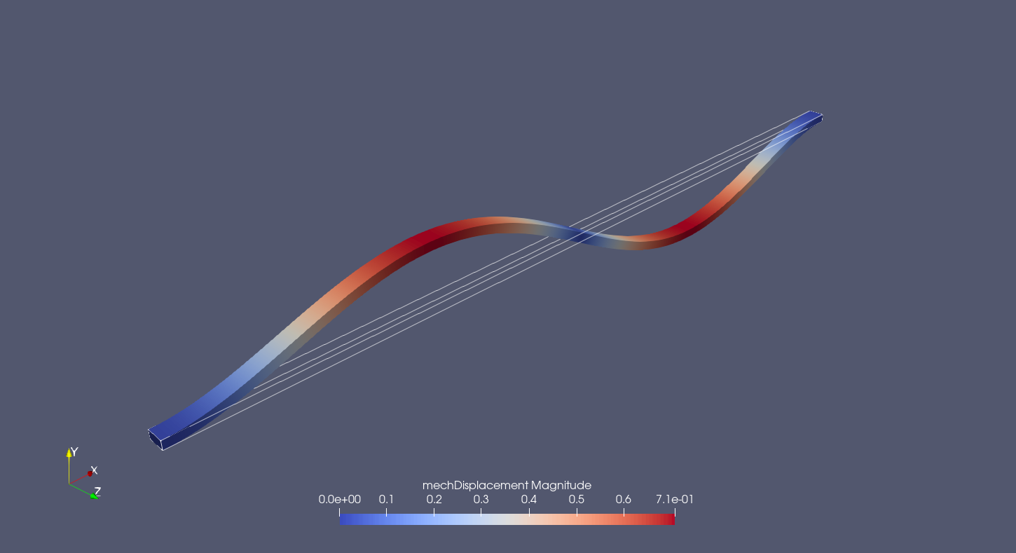
we can postprocess the results and compare the solutions. The postprocessing reveals the displacement of the centerline of the beam in y-direction. As an example the displacement of the centerline at the frequency of 778 Hz is plotted. The reduced model is capable of representing the global behaviour of the system, although the displacement at some points differ from the full model.

One can also repeat the harmonic simulations with more frequency steps in order to generate a transferfunction from the pressure to the x-displacement from the centerpoint on the centerline. The python script to generate the transfer function can be found here. Again the reduced model is capable of representing the system dynamics. The advantage of the reduced model is, that only a system of order 6 has to be solved every step. Depending on the dimensions of the full system this should faster than simulating the full system.

References

---

1. Clarence W De Silva. Vibration: fundamentals and practice. CRC Press, 2000. ↩

2. P. Koutsovasilis and M. Beitelschmidt. Comparison of model reduction techniques for large mechanical systems: a study on an elastic rod. Multibody system dynamics, 20:111–128, 2008. ↩

3. Michael Möser. Modalanalyse. Springer Berlin Heidelberg Imprint: Springer Vieweg, 2020. ↩